Map Specific Content and Value Information
DSM Data Descriptions
The table below describes the properties of the GLARS DSM elevation data.
| Format | Data is stored and distributed in 32 bit GeoTIFF file format with floating point elevation values. |
| Resolution | GLARS DSM strip and mosaic files are distributed at a ground sample distance (GSD) of 2 meters. |
| Coordinate System | GLARS DSM strip and mosaic files are projected in a local UTM zone (units: meters) depending on location and based on the WGS84 datum. |
| Vertical Reference | Vertical reference is height above the WGS84 ellipsoid. |
| Elevation Units | Elevation unit of measure is meters. |
| NULL Values (NoData) | Data may contain void pixels or regions over lakes, rivers, and other hydrographic features. Data voids may also be present where the source imagery contains cloud cover or shadowed areas. The void areas will contain null values (-9999) in lieu of the terrain elevations. |
| Metadata | Basic source material and production metadata is contained within the Esri shapefile and associated text files provided for each GLARS DSM strip and mosaic file. |
| Accuracy | Strips: 3.5 meters CE90 (Noh and Howat, 2015). Mosaic tile accuracy has not been assessed. |
DSM Strips
DSM Strip Download File Types
“dem.tif” – full data, with estimated surface elevation at each pixel. 32-bit GeoTIFF. Go here for in-depth information on how these were made. Further metadata listed in table below.
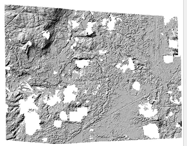
“dem browse.tif” – a gray-scale hillshade representation of the surface elevation data. Example:
“matchtag.tif” – Raster indicating DSM pixels derived from a stereo match (1) or those that have been interpolated (0).
“meta.txt” – DSM Strip metadata and metadata for the particular scenes used for that segment
“trans.mat” – Matlab file for workspace used in processing
DSM Strip Naming Convention
File naming of GLARS DSM strip files incorporate several elements related to the source material used to create the data. The example below describes the naming convention:
Key: SENSOR_DATE_STEREOIMAGE1_STEREOIMAGE2_SEGMENT_RESOLUTION_FILETYPE
Example: WV02_20150615_10300100443C2D00_1030010043373000_seg1_2m_dem
| SENSOR | DigitalGlobe satellite(s) that collected the stereopair image. Intrack pairs denoted by single sensor abbreviation (e.g. WV01). Crosstrack pairs denoted by a double sensor abbreviation (e.g. W1W2) |
| DATE | Date of earliest source stereopair image acquisition as YYYYMMDD. |
| STEREOIMAGE1 | DigitalGlobe Catalog ID number of the first stereopair image strip. |
| STEREOIMAGE2 | DigitalGlobe Catalog ID number of the second stereopair image strip. |
| SEGMENT | Segment of the DSM strip. |
| RESOLUTION | Ground sample distance (GSD) pixel size of the DSM in meters. |
| FILETYPE | Category of file included |
DSM Strip Delivery Contents
GLARS DSM strips are delivered as individual files. Note that the ortho geotiff files are not available in standard GLARS DSM products.
| *_dem.tif | A 32-bit floating point elevation raster. This is the primary GLARS DSM strip data file. |
| *_dem_browse.tif | An 8-bit, reduced resolution (10 m) hillshade representation of the strip. |
| *_matchtag.tif | Raster indicating DSM pixels derived from a stereo match (1) or those that have been interpolated (0). |
| *_meta.txt | Text file metadata document. |
| *_trans.mat | Matlab workspace file. |
DSM Mosaic Tiles
DSM Mosaic Tiling Schemes
GLARS DSM mosaic tiles maintain a planar projection because of their high resolution. To accommodate a projected coordinate system, mosaic tiling schemes were built for every UTM zone on a 100 km x 100 km grid. For the UTM South zones, the tiling grid begins with 01_01 at x=150,000, y=3,300,000 (-60.4°S) and ends with 67_07 at x=850,000, y=10,000,000 (equator) . UTM North tile grids begin with 01_01 at x=150,000, y=0 (equator) and end with 67_07 at x=850,000, y=6,700,000 (~60.4°N). Redundant tiles are removed where tiles from adjacent mosaic schemes overlap fully.
DSM Mosaic Tile Naming Convention
File naming of DSM mosaic files corresponds to the utm zone of the mosaic and the 100 km x 100 km utm-based tiling grid. These tiles are further subdivided into 50 km x 50 km sub-tiles for distribution at 2m.
Key: MOSAIC_TILE_SUBTILE_RESOLUTION_VERSION_FILETYPE
Example: utm10n_09_40_1_2_2m_v1.0_dem
| MOSAIC | Mosaic scheme denoted by utm zone |
| TILE | Tile index row and column |
| SUBTILE | Sub-tile index row and column if tiles are subdivided |
| RESOLUTION | Ground sample distance (GSD) pixel size of the DSM in meters |
| VERSION | Mosaic version |
| FILETYPE | Category of file included within the distributed tape archive (TAR) file |
DSM Mosaic Tile Delivery Contents
| index/*.shp | Esri shapefile, in WGS84 geographic coordinates, for the tile boundary. Includes metadata attributes. |
| *_browse.tif | 10m DSM hillshade |
| *_dem.tif | A 32-bit floating point elevation raster. This is the primary GLARS DSM tile datafile. |
| *_count.tif | number of contributing DSMs |
| *_countmt.tif | number of contributing DSMs excluding interpolated pixels |
| *_mad.tif | median absolute deviation of contributing DSMs |
| *_maxdate.tif | latest date of contributing DSMs in days since Jan 1, 2000 |
| *_mindate.tif | earliest date of contributing DSMs in days since Jan 1, 2000 |
| *_meta.txt | A metadata text file describing source imagery, creation date, registration sources and statistics. |
MTRI Inundation
These maps download as geotiff (EPSG 32615). Values at each pixel are
- 0 – dry
- 1 – open water
- 100 – emergent vegetation
MTRI Hydroperiod
These maps download as geotiff (EPSG 32615). Values at each pixel range:
- 0 – not wet
- 34 – consistently open water
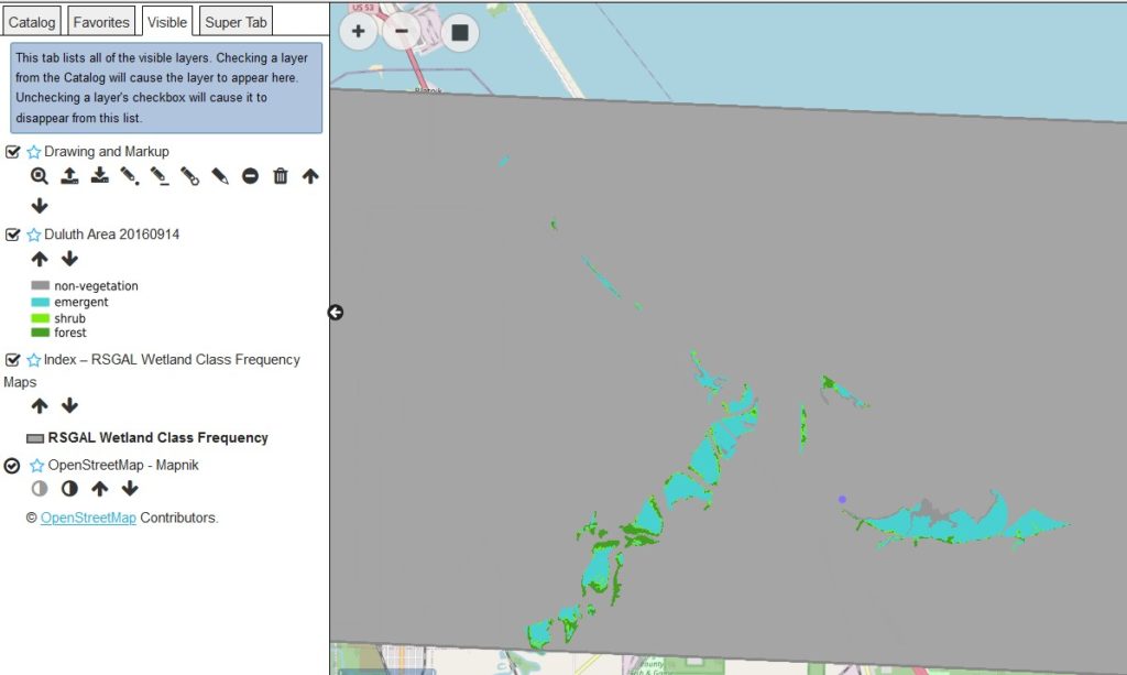
RSGAL Wetland Class by Date
- These maps show data only inside known wetland polygons.
- Turning on the Wetland Reference Dataset – 2004 GLCWC Coastal Wetlands may be useful for determining where to look for results in the output area.
- Leaving an index layer on as a neutral background also helps for finding areas with results.
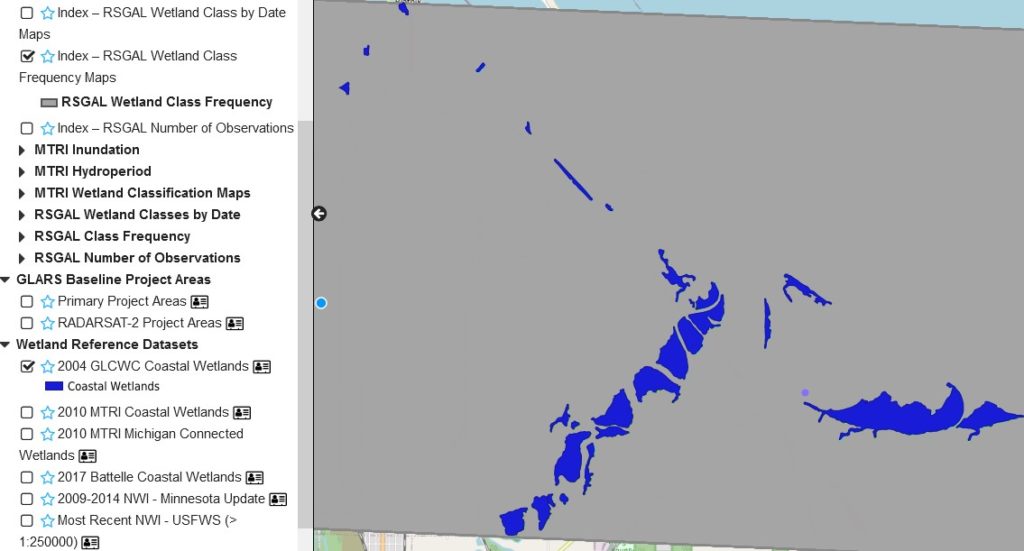
- Turn the index off to see results overlaid on photo or map background.
- These products download as geotiff, EPSG 6350. The values of each pixel are:
-
- – non-vegetation
- – emergent
- – shrub
- – forest
RSGAL Class Frequency
- These maps show the proportion of times each pixel is in each vegetation class over the number of photos available. For areas such as Duluth – West Superior, where data was collected frequently, this shows areas that were dominated by forest, shrub, or emergent, and areas where these classes changed most frequently.
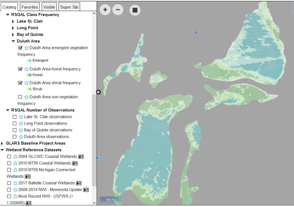
- Each vegetation type downloads as a separate geotif file so overlap areas can be evaluated.
- Files are EPSG 6350, and values at each pixel represent the proportion of times that pixel had the given vegetation value (0 to 1).
RSGAL Number of Observations
- This layer shows the depth of data used for the Class Frequency maps.
- This downloads as a single geotiff (EPSG 6350) and pixel values represent the number of photos used to make the Class Frequency analysis.